Hello Aliens...!!👋 ❤️

This article will introduce you to Unsupervised Learning and will help you gain a proper conceptual understanding of K-Means Clustering. So, without any further delay let's dive into the content.

Have you ever noticed how systemic books in the library are arranged? Like the maths section containing all maths books and references, the physics section consists of all physics references, and similarly, all the other subjects’ sections contain their books. We can say that all the books are grouped based on their subjects and arranged in the self.

Let me take another example, you might have visited the supermarket and observed how different items are arranged in different sections. Like you will never find groceries kept between clothes or grains kept between laundry material. Every item is perfectly arranged in its specific section.

These two are real-life examples of how items can be grouped or clustered based on a certain similarity.

So, from here I can conclude that clustering means the division of items into certain categories/sections or grouping them based on certain similarities.

There are some machine learning algorithms which follow the concept of clustering, K-means clustering algorithm is one of them.

Before we go further, let me define the name of this algorithm first.

What is K-means Clustering?

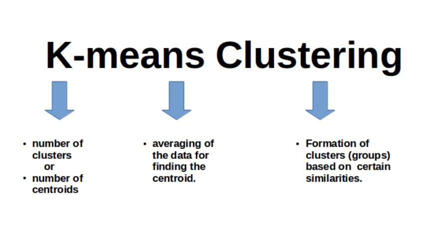
K-means algorithm is the unsupervised machine learning algorithm in which whole data is divided into K number of clusters. Every cluster has its centroid which is calculated by averaging the data points of that cluster. But what are the criteria of clustering?

• Inertia: It is the measure of intra-cluster distances, which means how far away the datapoint is concerning its centroid. This indicates that data points in the same cluster should be well matched and similar to each other. For better clustering, the inertia value should be minimum. In contrast, if the inertia value is high, that means data points in the cluster are not similar to each other. This indicates a simple concept that for a given datapoint intra-cluster distance should always be less than inter-cluster distance.
  

Advantages

1. Fast, robust and easier to understand.
2. Relatively efficient: O(tknd), where n is # objects, k is # clusters, d is # dimension of each object, and t is # iterations. Normally, k, t, d << n.
3. Gives best result when data set are distinct or well separated from each other.

Disadvantages

1. The learning algorithm requires apriori specification of the number of cluster centers.
2. The use of Exclusive Assignment - If there are two highly overlapping data then k-means will not be able to resolve that there are two clusters.
3. The learning algorithm is not invariant to non-linear transformations i.e. with different representation of data we get different results (data represented in form of cartesian co-ordinates and polar co-ordinates will give different results).
4. Euclidean distance measures can unequally weight underlying factors.
5. The learning algorithm provides the local optima of the squared error function.
6. Randomly choosing of the cluster center cannot lead us to the fruitful result. Pl
7. Applicable only when mean is defined i.e. fails for categorical data.
8. Unable to handle noisy data and outliers.
9. Algorithm fails for non-linear data set.

How does K – means algorithm works?

1. Initialize ‘ K’ and centroid values.
   
2. Assign data points to the closest clusters, by calculating the Euclidean distance.
   
3. When the clusters are formed, recompute their centroid values by calculating the average of data points.
   
4. Repeat steps 2 & 3 until all the clusters are stable.
   

Cool, isn’t it? Let’s visualize these steps for better understanding.

Suppose we have a dataset, Let’s start with plotting the data points.

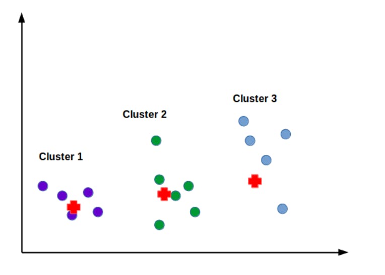
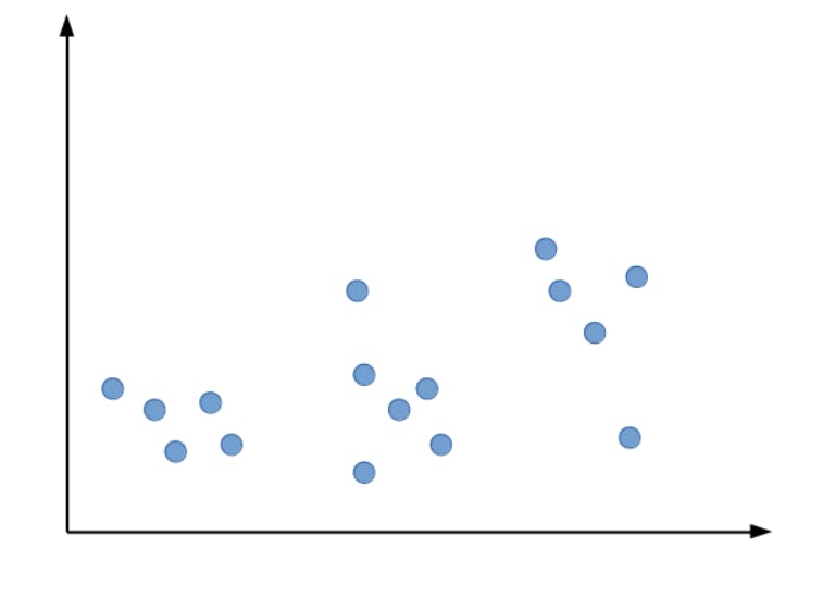As we can see the given data points can be roughly divided into three clusters. Let our K value be 3. Now, let’s initialize the centroids randomly.

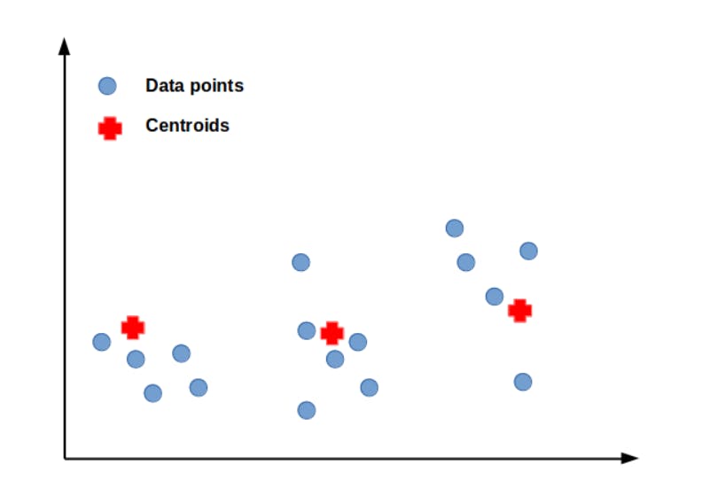
As we have marked our centroid values. The next step is to assign the data points to the nearest cluster. This is done by calculating the distance between the centroids and data points. Euclidean distance is a better choice when the need is to find the shortest distance.

Euclidean distance can be defined as :

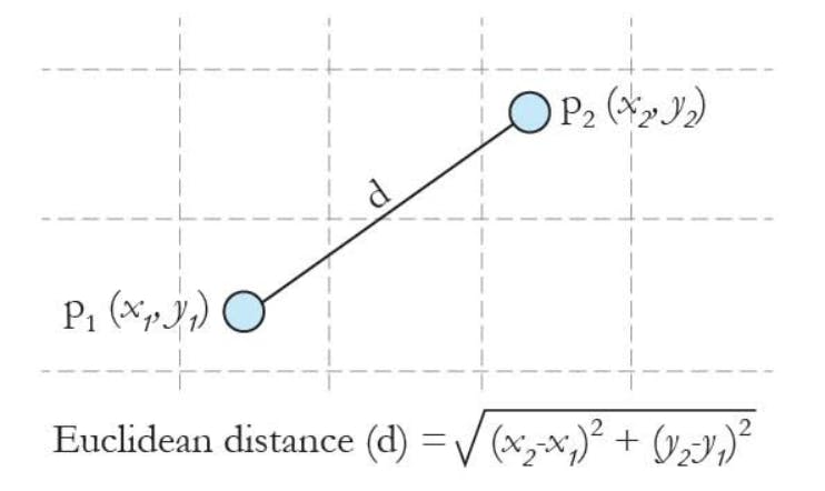
The below picture shows how we can use Euclidean distance and assign clusters to the data points.

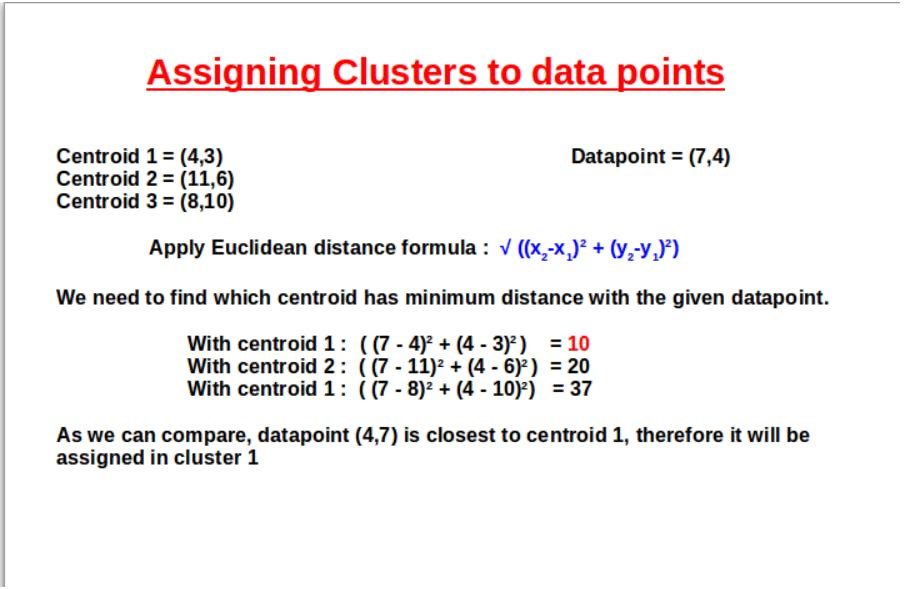
Similarly, Euclidean distance is calculated for every data point. After the formation of clusters, the next step is to update or recompute the centroid values. This is done by taking the Euclideanaverage or mean value of the data points in a particular cluster.

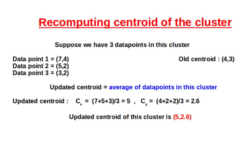
After updating the centroids, we need to repeat the last two steps. This is because since our centroid value has changed, there might be changes in the Euclidean distance calculated. Therefore, some data points might change their clusters as we recompute the euclidean distance and update the clusters.

This seems like this isn’t a 4 step process. It might take certain iterations to form stable clusters. So, how do we know when to stop performing these steps.

Stopping criteria?

1. We can stop our training when even after many iterations our centroids are stable, that is they are the same and fixed.
2. We can stop our training when even after many iterations our data points remain in the same cluster. That they do not change their cluster anymore.
3. We can stop our training when the fixed or maximum number of iterations is reached. This is because an insufficient number of iterations might give us poor results and hence unstable clusters.
   

After the formation of stable clusters. Let’s visualize how our data points look.

Looks great, isn’t it? I guess reading this blog till now, one question would have crossed your mind. If I am not wrong, the question is “How can we choose k value in case of real problems, where the dataset consists of thousands of data points?’’

Alright, don’t stress yourself. I will explain everything to you in detail.

How to choose the optimal ‘K’?

‘K’ in K-means clustering has an important role. Wrong k value might result in wrong or unstable clusters. So, choosing the optimal value of k is a tough task.

Two methods can be used for choosing the right value of K.

• Elbow method

• The Silhouette Method
  

Let’s understand them one by one.

Elbow method

In the elbow method, we plot WSS error against different values of K.

WSS error, isn’t it a new term for you? Let’s crack this.

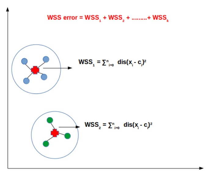
WSS error is the Within-cluster sum of squared error.

• Take a cluster(say cluster 1); Find the distance between a data point and its centroid(within-cluster distance)

• Do this for every data point in that cluster

• Sum the values, Consider this summation as WSS1

• Find such summation for every cluster.

• Finally, sum up these values to get the WSS error.
  

Refer to the diagram for a, more clear understanding.

After finding the WSS error, plot it against the different values of K.

But why did we call it an elbow method?

This is because when we will plot WSS errors against different values of K. We will see the graph in the shape of an elbow. The value of K where we can see the clear arm will be our optimal K.

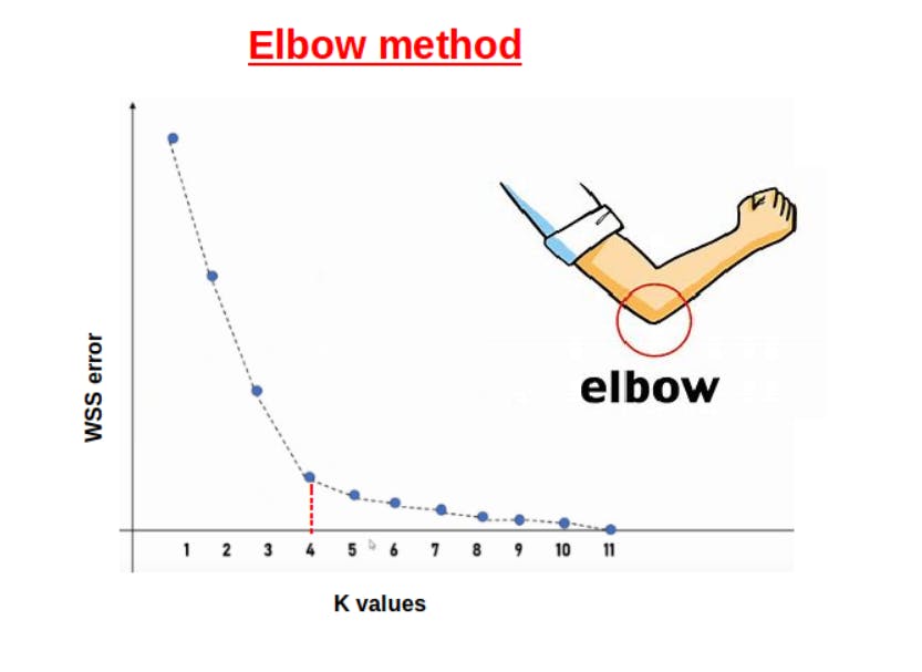
So, as in the above figure, our optimal k value is 4.

But sometimes we might not get a clear elbow, by this method. At that time, we can use the Silhouette Method.

Silhouette method

The silhouette method can be considered as a better technique for finding an optimal value of K or simply a validation technique for clustering algorithms.

In this method, we need to find the average intra-cluster distance and the minimum average inter-cluster distance.

Formula for the silhouette coefficient can be written as :

                 s(i) =( b(i) – a(i) ) /  max(b(i),a(i))                   

Let’s understand this formula, with the help of a diagram

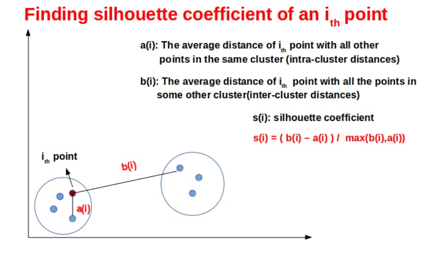
The range of silhouette coefficient is (-1,1)

If the coefficient value is closer to 1, that means the point is similar to all other points in the same cluster.

If the coefficient value is closer to -1, that means the point is highly dissimilar with others of its cluster and assigned in the wrong cluster

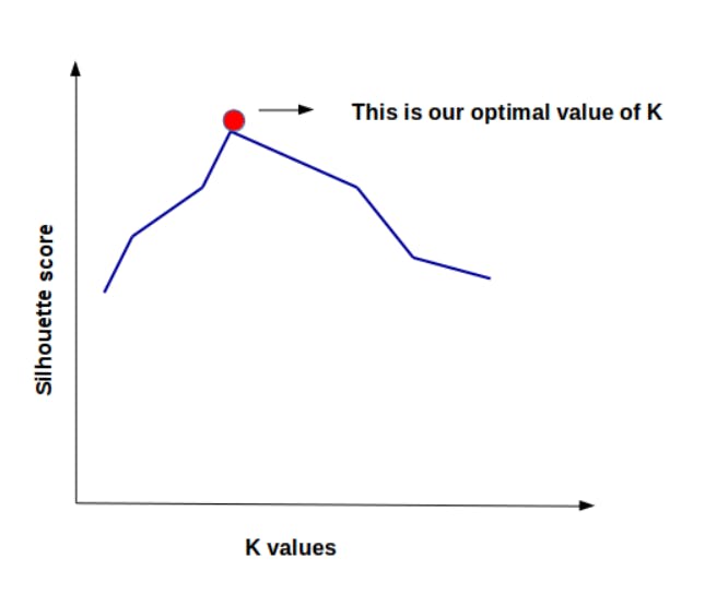
After calculation of the silhouette coefficient, we can plot the silhouette score against different k values.

The value of K at which there is a peak in the graph is considered as optimal k.

It can be visualized as :

I hope you have understood these two methods. There are even more such methods to find the optimal value of k in clustering algorithms. But these two are most commonly used. You can use the elbow method to find the optimal k, but if the result is not clear from this method then you can try to validate it with the silhouette method.

Now as we have learned the whole concept behind k-means clustering. Let’s learn how to implement this through python’s in-built libraries.

Code Implementation

I am taking a very simple dataset here, with a few rows and columns, for better understanding. So, let’s get started. You can find the dataset here .

Gathering data

#loading required libraries
import pandas as pd
from matplotlib import pyplot as plt
%matplotlib inline
#reading csv file with pandas
df = pd.read_csv("data.csv")
#the column was irrelevant, so i dropped it
df = df.drop(df.columns[0],axis=1)
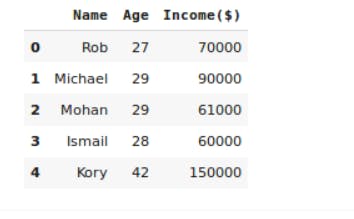
#print the first five rows of dataset
df.head()

Output:

Scaling the data

#importing the library for feature scaling
from sklearn.preprocessing import MinMaxScaler
scaler = MinMaxScaler()
#feature scaling on income column
scaler.fit(df[['Income($)']])
df['Income($)'] = scaler.transform(df[['Income($)']])
#feature scaling on Age column
scaler.fit(df[['Age']])
df['Age'] = scaler.transform(df[['Age']])
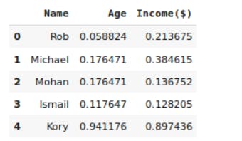
#printing first 5 rows our updated dataset
df.head()
#we have not done feature scaling on the name column as it will not be required in next steps, and it isn't a numerical value
#range of every value in the columns income and age will be (0,1)

Output:

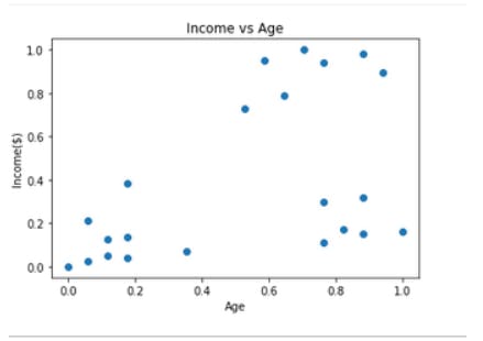
Visualizing the data

#plotting Income vs age graph
plt.scatter(df.Age,df['Income($)'])
plt.xlabel('Age')
plt.ylabel('Income($)')
plt.title('Income vs Age')
plt.show()

Output:

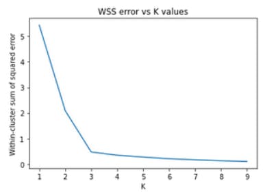
Using Elbow method to find optimal ‘k’

#import required library
from sklearn.cluster import KMeans
#create a list 
wss = []
#deciding k range-here the dataset has few rows thats why i am taking k range (1,10)
k_rng = range(1,10)
#perform iterations
for k in k_rng:
    km = KMeans(n_clusters=k)
    km.fit(df[['Age','Income($)']])
    wss.append(km.inertia_)

plt.xlabel('K')
plt.ylabel('Within-cluster sum of squared error')
plt.title('WSS error vs K values')
plt.plot(k_rng,sse)

Output:

Fit the K-means model

# Fitting K-Means to the dataset
kmeans = KMeans(n_clusters=3) #we can see elbow at k=3 in the above graph
#fit the model 
y_predicted = kmeans.fit_predict(df[['Age','Income($)']])
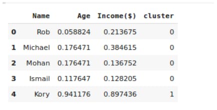
#create a new column named cluster to store the predicted values
df['cluster']=y_predicted
#lets see how our model has predicted and assigned clusters to the datapoints
df.head()

Output:

Visualizing the final clusters

df1 = df[df.cluster==0]
df2 = df[df.cluster==1]
df3 = df[df.cluster==2]
plt.scatter(df1.Age,df1['Income($)'],color='green',label = 'Cluster 1')
plt.scatter(df2.Age,df2['Income($)'],color='red',label = 'Cluster 2')
plt.scatter(df3.Age,df3['Income($)'],color='black',label = 'Cluster 3')
plt.scatter(kmeans.cluster_centers_[:,0],kmeans.cluster_centers_[:,1],color='blue',marker='*',label='centroid')
plt.xlabel('Age')
plt.ylabel('Income ($)')
plt.title('Final clusters')
plt.legend()
plt.show()

Output:

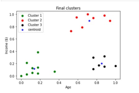
So this is how the K-means clustering algorithm works.

An example in Sklearn

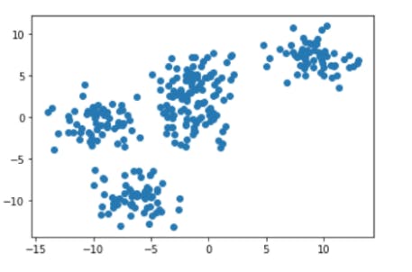
1. Generate “random” clusters with sklearn’s "make_blobs".

from sklearn.datasets import make_blobs
import matplotlib.pyplot as plt
data = make_blobs(
    n_samples=300, 
    n_features=2, 
    centers=5, 
    cluster_std=1.75, 
    random_state=11
)
plt.scatter(data[0][:,0], data[0][:,1])

Output:

2. Import and run K-Means

from sklearn.cluster import KMeans
kmeans = KMeans(n_clusters=5)
kmeans.fit(data[0])
y = kmeans.fit_predict(data[0])

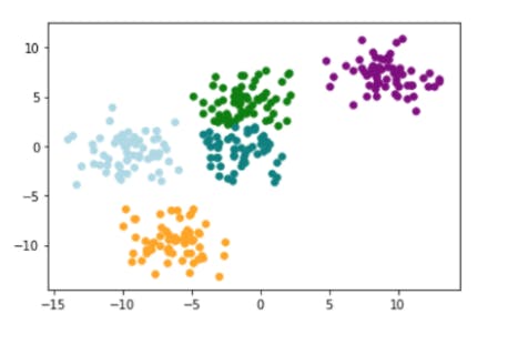
3. Plot clusters

for idx,color in enumerate(['green','lightblue','orange','purple','teal']):
    plt.scatter(
        points[y ==idx,0], 
        points[y == idx,1], 
        s=30, 
        c=color
    )

Output:

Conclusion

In this blog, we have learned how the K-means algorithm works, what is the clustering criteria for this, how to choose the optimal K, how to validate the K(silhouette method), and at last we have learned how to implement this algorithm with the help of in-built libraries.

I have used a very simple dataset, remember real problems will never be like this. Problem dataset may contain many columns and rows. There you will be required to choose features that are relevant in finding the final predictions. This was just an example to make you understand how things work here. So, try to build your own k-means model with a different dataset.

Huzza...!!Hope that, today you learned something new😊

Thank you for reading till the end. Like to be friends, connect me through Twitter , GitHub , LinkedIn